
関連するソリューション

業務改革
AI
テクニカルスペシャリスト
松尾 大輔 
今回は、以前から気になっていたRaspberry Pi AI Camera(以降、AI Camera)を用いて、エッジAIシステムを構築してみました。
AI Cameraとは、IMX500というAI処理を行うイメージセンターが搭載されたカメラです。
Raspberry Pi AI Camera
1.AI cameraのセットアップ
はじめに、Raspberry PiとAI Cameraを接続します。Raspberry Pi 5の場合は、AI Cameraのケーブルを、同梱されている先の細いケーブルに、差し替える必要があります。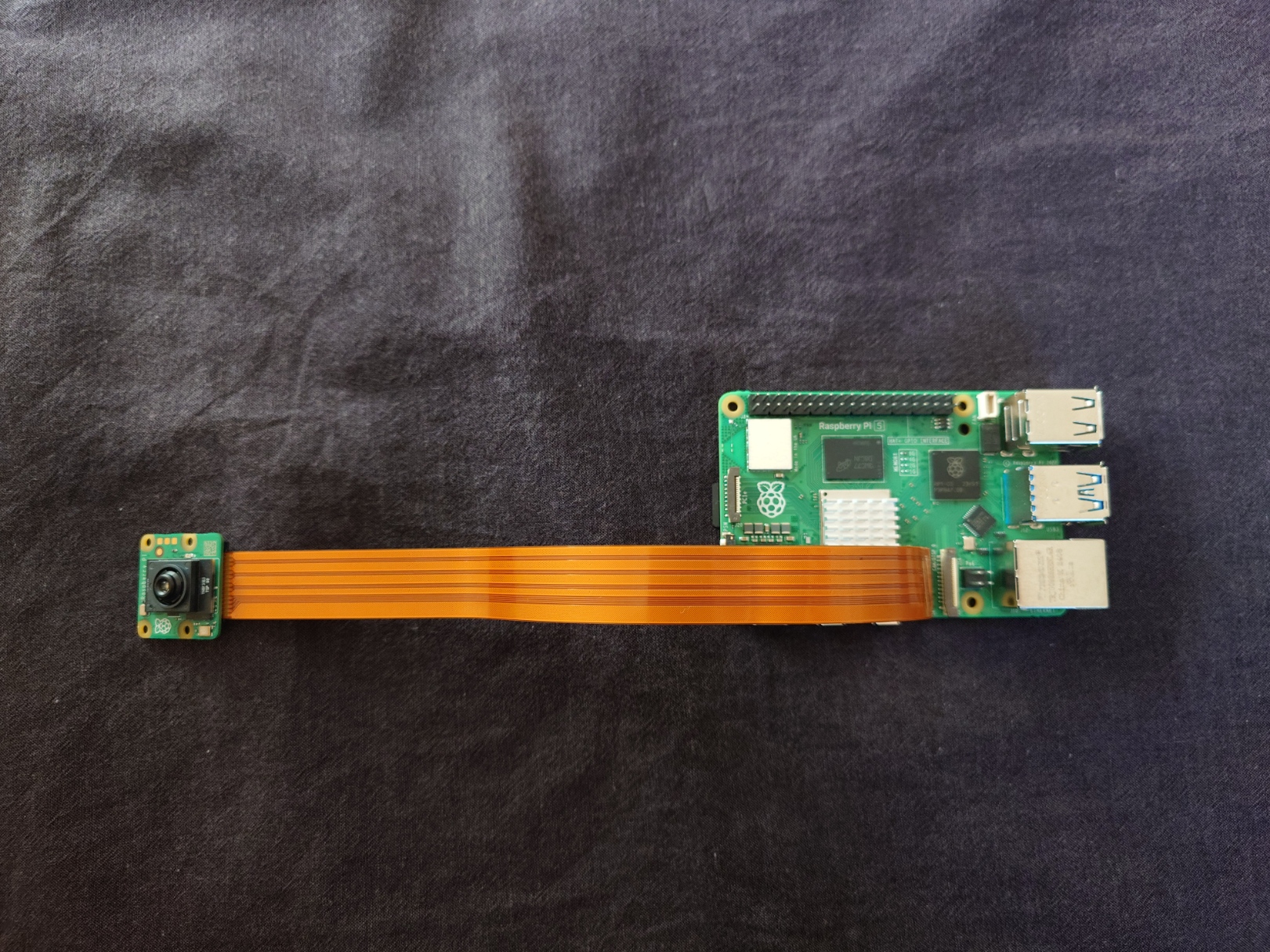 Raspberry Pi 5にAI Cameraを接続
次に、以下に記載されている手順に従ってセットアップを行います。
https://www.raspberrypi.com/documentation/accessories/ai-camera.html
まず、Raspberry Piを最新の状態にします。
$ sudo apt update && sudo apt full-upgradeIMX500のファームウェアをインストールします。
$ sudo apt install imx500-allRaspberry Piを再起動します。
$ sudo reboot再起動したら、AI Camera (IMX500) が認識されていることを確認します。
$ sudo dmesg | grep imx500
[    0.419205] platform 1f00128000.csi: Fixed dependency cycle(s) with /axi/pcie@120000/rp1/i2c@80000/imx500@1a
[    3.075421] rp1-cfe 1f00128000.csi: found subdevice /axi/pcie@120000/rp1/i2c@80000/imx500@1a
[    3.415697] imx500 11-001a: Device found is imx500
[    3.416234] rp1-cfe 1f00128000.csi: Using sensor imx500 11-001a for capture
AI Cameraに初めから入っている MobileNet-SSDで動作確認をします。
$ rpicam-hello -t 0s --post-process-file /usr/share/rpi-camera-assets/imx500_mobilenet_ssd.json --viewfinder-width 1920 --viewfinder-height 1080 --framerate 30
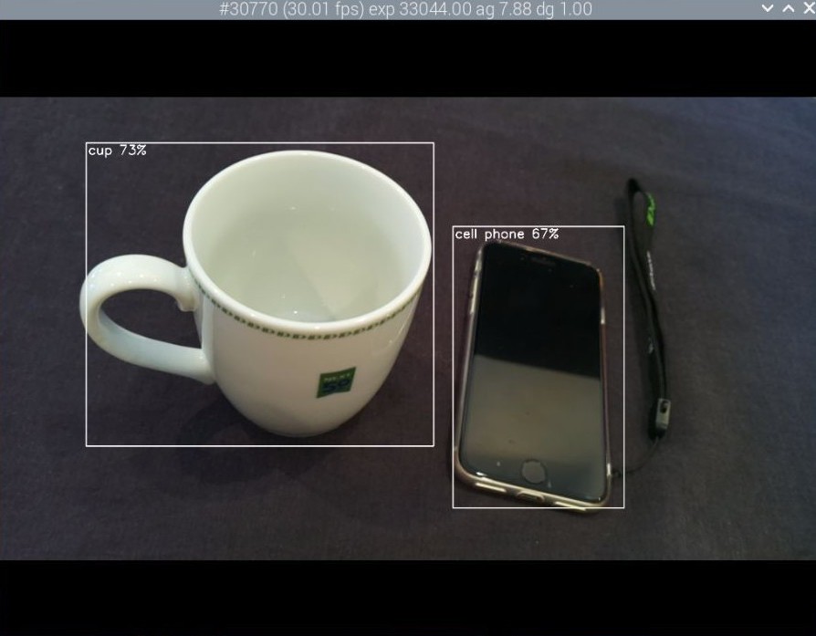 物体検知の実行
この状態でも物体検知ができていることが確認できますね。
2.独自モデルの構築
実使用においては、独自のモデルを構築してAI Cameraにデプロイすることが多いかと思います。その際は、独自モデルをPC上で作成し、それをAI Cameraで実行できる形式にコンバートして、デプロイします。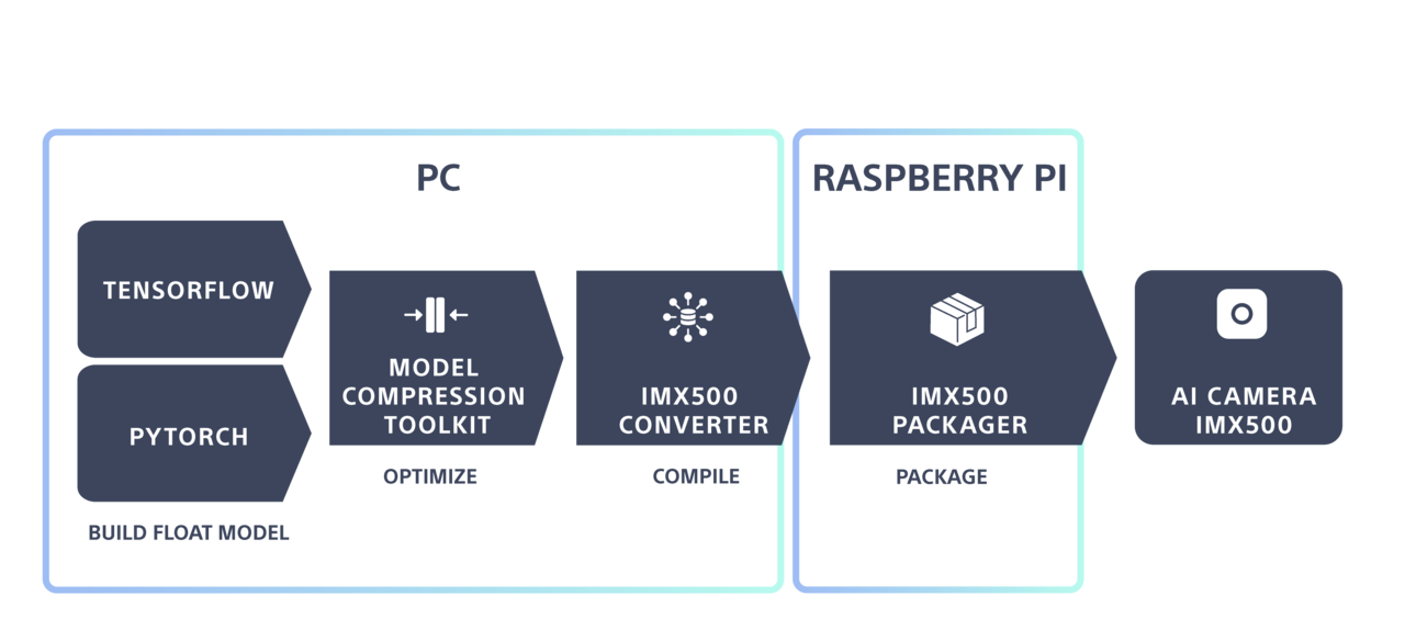
引用: https://developer.aitrios.sony-semicon.com/en/raspberrypi-ai-camera/develop/ai-tutorials/prepare-and-deploy-ai-models-tutorial
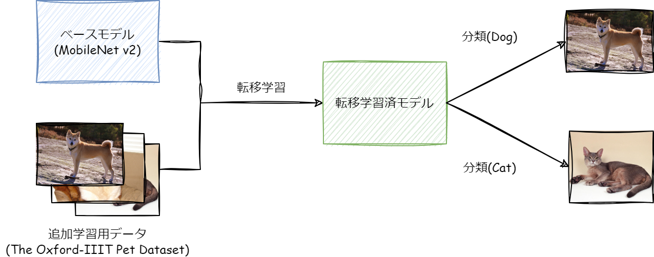
今回は独自モデルの例として、学習済みのMobileNetに転移学習を行います。以下のオープンデータセットを追加学習用データとして使用し、犬と猫の画像を分類するモデルを作成します。
The Oxford-IIIT Pet Dataset
■作成するモデルのイメージ
以降は、Pythonのコード例となりますが、Google ColaboratoryなどのNotebook上での逐次実行を想定しています。
データセットの準備
データセットの読み込みは、PyTorchのImageFolderを使用します。入手したデータセットのディレクトリ構成を、ImageFolderで読み込ませるための構成に変更します。■ディレクトリ構成のイメージ
dataset/
├── train/
│   ├── cat/
│   │   ├── Abyssinian_1.jpg
│   │   ├── Bengal_23.jpg
│   │   └── ...
│   └── dog/
│       ├── Beagle_45.jpg
│       ├── Boxer_12.jpg
│       └── ...
└── val/
    ├── cat/
    └── dog/
■コード
import os
import shutil
from sklearn.model_selection import train_test_split
import re

def organize_dataset(source_dir, dest_dir, val_split=0.2):
    """
    ファイル名に基づいて画像を猫(cat)と犬(dog)のクラスに分類してデータセットを構築

    Parameters:
        source_dir: 元の画像があるディレクトリ(すべての画像が1つのフォルダにある)
        dest_dir: データセットを作成するディレクトリ
        val_split: 検証データの割合
    """
    # 猫の品種リスト
    cat_breeds = {
        "abyssinian", "bengal", "birman", "bombay", "british_shorthair",
        "egyptian_mau", "maine_coon", "persian", "ragdoll", "russian_blue",
        "siamese", "sphynx"
    }

    # 画像ファイルの一覧を取得
    image_files = [f for f in os.listdir(source_dir)
                    if f.lower().endswith((".jpg", ".jpeg", ".png", ".bmp"))]

    # ファイル名からクラス(猫/犬)を判定
    class_images = {"cat": [], "dog": []}
    for img in image_files:
        # 拡張子を除去
        name_without_ext = os.path.splitext(img)[0]
        # 末尾の連番を除去(末尾の数字を削除)
        breed_name = re.sub(r"\d+$", "", name_without_ext).rstrip("_").rstrip("-").lower()

        # 品種名から猫/犬を判定
        if any(cat_breed in breed_name for cat_breed in cat_breeds):
            class_images["cat"].append(img)
        else:
            class_images["dog"].append(img)

    # クラスごとにディレクトリを作成し、画像を振り分け
    for class_name, images in class_images.items():
        # trainとvalディレクトリにクラスのサブディレクトリを作成
        train_class_dir = os.path.join(dest_dir, "train", class_name)
        val_class_dir = os.path.join(dest_dir, "val", class_name)
        os.makedirs(train_class_dir, exist_ok=True)
        os.makedirs(val_class_dir, exist_ok=True)

        # trainとvalに分割
        train_images, val_images = train_test_split(
            images,
            test_size=val_split,
            random_state=42
        )

        # 画像をコピー
        for img in train_images:
            src = os.path.join(source_dir, img)
            dst = os.path.join(train_class_dir, img)
            shutil.copy2(src, dst)

        for img in val_images:
            src = os.path.join(source_dir, img)
            dst = os.path.join(val_class_dir, img)
            shutil.copy2(src, dst)

        print(f"Class {class_name}: {len(train_images)} training images, {len(val_images)} validation images")
■実行例
base_dir = "dataset"
source_dir = "original_images"  # すべての画像が入っているディレクトリ

# ディレクトリ構造を作成
os.makedirs(os.path.join(base_dir, "train"), exist_ok=True)
os.makedirs(os.path.join(base_dir, "val"), exist_ok=True)

# 画像を分類して配置
organize_dataset(source_dir, base_dir, val_split=0.2)
独自モデルの準備
ここからは、実際にモデルを実装していきます。ステップごとに関数を作成して、最後にそれを実行します。(1) ライブラリの準備
!pip install -q torch torchvision
!pip install -q onnx==1.16.1
import importlib
if not importlib.util.find_spec("model_compression_toolkit"):
!pip install model_compression_toolkitimport torch
import torch.nn as nn
import torch.optim as optim
from torch.utils.data import DataLoader
from torchvision.models import mobilenet_v2, MobileNet_V2_Weights
from torchvision import transforms, datasets
import numpy as np
import random
from tqdm import tqdm
import model_compression_toolkit as mct
import os(2)データセットの読み込み
「2.1 データセットの準備」で用意したデータセットを読み込みます。
def create_data_loaders(train_dir, val_dir, batch_size=32):
    """
    転移学習用のデータローダーを作成

    Parameters:
        train_dir (str): 学習データのディレクトリパス
        val_dir (str): 検証データのディレクトリパス
        batch_size (int): バッチサイズ
    """
    # データ拡張と前処理の定義
    train_transform = transforms.Compose([
        transforms.Resize(256),
        transforms.RandomResizedCrop(224),
        transforms.RandomHorizontalFlip(),
        transforms.ColorJitter(brightness=0.2, contrast=0.2, saturation=0.2),
        transforms.ToTensor(),
        transforms.Normalize([0.485, 0.456, 0.406], [0.229, 0.224, 0.225])
    ])

    val_transform = transforms.Compose([
        transforms.Resize(256),
        transforms.CenterCrop(224),
        transforms.ToTensor(),
        transforms.Normalize([0.485, 0.456, 0.406], [0.229, 0.224, 0.225])
    ])

    # データセットの作成
    train_dataset = datasets.ImageFolder(train_dir, transform=train_transform)
    val_dataset = datasets.ImageFolder(val_dir, transform=val_transform)

    # データローダーの作成
    train_loader = DataLoader(
        train_dataset,
        batch_size=batch_size,
        shuffle=True,
        num_workers=4,
        pin_memory=True
    )

    val_loader = DataLoader(
        val_dataset,
        batch_size=batch_size,
        shuffle=False,
        num_workers=4,
        pin_memory=True
    )

    return train_loader, val_loader, len(train_dataset.classes)
(3)モデルの準備
事前学習済みモデルの読み込みと、転移学習用の修正です。def prepare_model_for_transfer_learning(num_classes, freeze_backbone=True):
"""
転移学習用のMobileNetV2モデルを準備
Parameters:
num_classes (int): 新しいタスクのクラス数
freeze_backbone (bool): バックボーンを凍結するかどうか
"""
# 事前学習済みモデルの読み込み
weights = MobileNet_V2_Weights.IMAGENET1K_V2
model = mobilenet_v2(weights=weights)
if freeze_backbone:
# バックボーン部分のパラメータを凍結
for param in model.parameters():
param.requires_grad = False
# 分類層を新しいタスク用に置き換え
in_features = model.classifier[-1].in_features
model.classifier = nn.Sequential(
nn.Dropout(p=0.2),
nn.Linear(in_features, num_classes)
)
return model
(4) 転移学習の実行
転移学習部分は、PyTorchを用いた標準的な実装です。def train_model(model, train_loader, val_loader, num_epochs=10):
"""
モデルの転移学習を実行
Parameters:
model: 学習するモデル
train_loader: 学習データのDataLoader
val_loader: 検証データのDataLoader
num_epochs (int): エポック数
"""
device = torch.device("cuda:0" if torch.cuda.is_available() else "cpu")
model = model.to(device)
criterion = nn.CrossEntropyLoss()
# 分類層のパラメータのみを最適化
optimizer = optim.Adam(model.classifier.parameters(), lr=0.001)
scheduler = optim.lr_scheduler.ReduceLROnPlateau(
optimizer,
mode="min",
patience=2,
factor=0.1
)
best_val_loss = float("inf")
best_model_state = None
for epoch in range(num_epochs):
# 学習フェーズ
model.train()
train_loss = 0.0
train_correct = 0
train_total = 0
for inputs, labels in tqdm(train_loader, desc=f"Epoch {epoch+1}/{num_epochs}"):
inputs, labels = inputs.to(device), labels.to(device)
optimizer.zero_grad()
outputs = model(inputs)
loss = criterion(outputs, labels)
loss.backward()
optimizer.step()
train_loss += loss.item()
_, predicted = outputs.max(1)
train_total += labels.size(0)
train_correct += predicted.eq(labels).sum().item()
train_loss = train_loss / len(train_loader)
train_acc = 100. * train_correct / train_total
# 評価フェーズ
model.eval()
val_loss = 0.0
val_correct = 0
val_total = 0
with torch.no_grad():
for inputs, labels in val_loader:
inputs, labels = inputs.to(device), labels.to(device)
outputs = model(inputs)
loss = criterion(outputs, labels)
val_loss += loss.item()
_, predicted = outputs.max(1)
val_total += labels.size(0)
val_correct += predicted.eq(labels).sum().item()
val_loss = val_loss / len(val_loader)
val_acc = 100. * val_correct / val_total
# 学習率の調整
scheduler.step(val_loss)
# ベストモデルの保存
if val_loss < best_val_loss:
best_val_loss = val_loss
best_model_state = model.state_dict()
print(f"Epoch {epoch+1}/{num_epochs}:")
print(f"Train Loss: {train_loss:.4f}, Train Acc: {train_acc:.2f}%")
print(f"Val Loss: {val_loss:.4f}, Val Acc: {val_acc:.2f}%")
# ベストモデルの復元
model.load_state_dict(best_model_state)
return model
(5)モデルの評価(転移学習後、モデルの量子化後)
モデルの評価部分です。転移学習後のモデルと、それを量子化した後のモデル双方を評価します。def evaluate_model(model, test_loader):
"""
モデルの評価
Parameters:
model: 評価するモデル
test_loader: 評価データのDataLoader
"""
device = torch.device("cuda:0" if torch.cuda.is_available() else "cpu")
model.to(device)
model.eval()
correct = 0
total = 0
with torch.no_grad():
for data in tqdm(test_loader, desc="Evaluating"):
images, labels = data
images, labels = images.to(device), labels.to(device)
outputs = model(images)
_, predicted = outputs.max(1)
total += labels.size(0)
correct += predicted.eq(labels).sum().item()
accuracy = 100. * correct / total
print(f"Accuracy: {accuracy:.2f}%")
return accuracy
(6)モデルの量子化
モデルを量子化する部分です。def quantize_model(model, train_loader, n_iter=10):
"""
モデルの量子化を実行
Parameters:
model: 量子化するモデル
train_loader: 学習データのDataLoader
n_iter (int): 代表的なデータセットのサイズ
"""
def representative_dataset_gen():
dataloader_iter = iter(train_loader)
for _ in range(n_iter):
yield [next(dataloader_iter)[0]]
# TPCの取得
target_platform_cap = mct.get_target_platform_capabilities("pytorch", "default")
# Post-Training Quantizationの実行
quantized_model, quantization_info = mct.ptq.pytorch_post_training_quantization(
in_module=model,
representative_data_gen=representative_dataset_gen,
target_platform_capabilities=target_platform_cap
)
return quantized_model
(7)メインの実行フロー
ここまでで実装した関数を実行していきます。def main():
# パラメータの設定
train_dir = "<DATASET PATH>/train" # 学習データのパス
val_dir = "<DATASET PATH>/val" # 検証データのパス
batch_size = 32
num_epochs = 10
# 1. データローダーの準備
train_loader, val_loader, num_classes = create_data_loaders(
train_dir,
val_dir,
batch_size
)
# 2. モデルの準備
model = prepare_model_for_transfer_learning(
num_classes,
freeze_backbone=True
)
# 3. 転移学習の実行
print("Starting transfer learning...")
trained_model = train_model(
model,
train_loader,
val_loader,
num_epochs
)
# 4. 転移学習後のモデル評価
print("\nEvaluating transfer learned model:")
float_accuracy = evaluate_model(trained_model, val_loader)
# 5. モデルの量子化
print("\nQuantizing model...")
quantized_model = quantize_model(trained_model, train_loader)
# 6. 量子化モデルの評価
print("\nEvaluating quantized model:")
quantized_accuracy = evaluate_model(quantized_model, val_loader)
# 7. モデルのエクスポート
print("\nExporting model...")
def representative_dataset_gen():
dataloader_iter = iter(train_loader)
for _ in range(10):
yield [next(dataloader_iter)[0]]
mct.exporter.pytorch_export_model(
quantized_model,
save_model_path="quantized_transfer_model.onnx",
repr_dataset=representative_dataset_gen
)
print("\nResults summary:")
print(f"Original model accuracy: {float_accuracy:.2f}%")
print(f"Quantized model accuracy: {quantized_accuracy:.2f}%")
print("Model exported as 'quantized_transfer_model.onnx'")
if __name__ == "__main__":
main()
実行したところ、量子化前後で精度はそれほど変わりませんでした。
Results summary:
Original model accuracy: 98.71%
Quantized model accuracy: 98.51%
Model exported as 'quantized_transfer_model.onnx'
3.独自モデルをRaspberry Piへデプロイ
Raspberry PI へのデプロイは、以下のサイトの手順を参考に実施します。前半はPCで実施し、後半はRaspberry Piで実施します。https://developer.aitrios.sony-semicon.com/en/raspberrypi-ai-camera/develop/ai-tutorials/prepare-and-deploy-ai-models-tutorial?version=2024-11-21&progLang=
コンバート(PC)
サイトの「2.1.3. Compile with IMX500 Converter」を参考に、量子化したモデルを、AI Cameraで実行できる形式にコンバートします。しかし、この手順はWindowsでは実行できないため、WSLなどのLinux環境で実行する必要があります。また、Javaのインストールも必要です。
$ pip install imx500-converter[pt]
$ imxconv-pt -i <MODEL PATH> -o <CONVERTER OUTPUT PATH> --overwrite-output
<CONVERTER OUTPUT PATH>に、packerOut.zipというファイルが生成されるので、これをRaspberry Piに格納します。
さらに、以下のような分類するクラスを記入したファイル(class.txt)を作成して格納します。
cat
dog
パッケージ化(Raspberry Pi)
サイトの「2.2.3. Package model」を参考にパッケージ化を行います(2.2.1. ~ 2.2.2.は、これまでの手順にて実行済みです)。$ sudo apt install python3-opencv python3-munkres
$ imx500-package -i <CONVERTER OUTPUT PATH> -o <RPK OUTPUT PATH>実行(Raspberry Pi)
サイトの「2.2.4. Visualize model」を参考に実行してみます。$ git clone https://github.com/raspberrypi/picamera2.git実行に使用するプログラムですが、2クラス分類の場合は、そのまま実行するとエラーとなるため、コピーして編集します。
$ cp picamera2/examples/imx500/imx500_classification_demo.py classification.pyコピーしたclassification.pyを以下のように編集します。
# 30行目:コメントアウトします。
# assert len(LABELS) in [1000, 1001], "Labels file should contain 1000 or 1001 labels."

# 52行目:以下のように変更します。
top_indices = np.argpartition(-np_output, 1)[:2]
プログラムを実行します。
$ python classification.py --model <RPK OUTPUT PATH>/network.rpk --preserve-aspect-ratio --label class.txt --softmax
リアルタイムで画像分類が行われます。dogが0.986(98.6%)となっているので、正しく分類できていることが分かりますね。
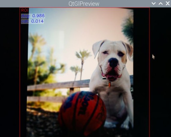
画像分類の結果
まとめ
実機上では、リアルタイム映像を瞬時に推論しており、スピードの速さに驚きました。しかし、ワークロードによっては、実機上の精度が低下することもあり、実務では深い検証が必要になると思います。今回の検証においても、はじめは犬と猫の37種別を分類するモデルで検証しましたが、実機上の精度が上がらず、犬と猫の2クラス分類に変更しました。これらを考慮しても、AIの処理をカメラに任せることができるため、Raspberry Pi本体は、温度センサーなどのセンサー制御や、管理用のWebアプリの実行といった別の処理に専念させることができます。これは大きなメリットだと思います。エッジAIの可能性が多いに広がるのではないかと感じました。
以上、最後までお読みいただきありがとうございました。
当サイトの内容、テキスト、画像等の転載・転記・使用する場合は問い合わせよりご連絡下さい。
エンジニアによるコラムやIDグループからのお知らせなどを
メルマガでお届けしています。